XLM-E: XLM via ELECTRA
XLM-E stands for “Cross-lingual Language Modeling via Electra” which is a cross-lingual language model that was pre-trained on two ELECTRA-style tasks as we are going to see later. XLM-E was proposed by Microsoft in 2021 and published in their paper: Cross-lingual Language Model Pre-training via ELECTRA. The official code for this paper can be found on Microsoft’s GitHub repository: microsoft/unilm.
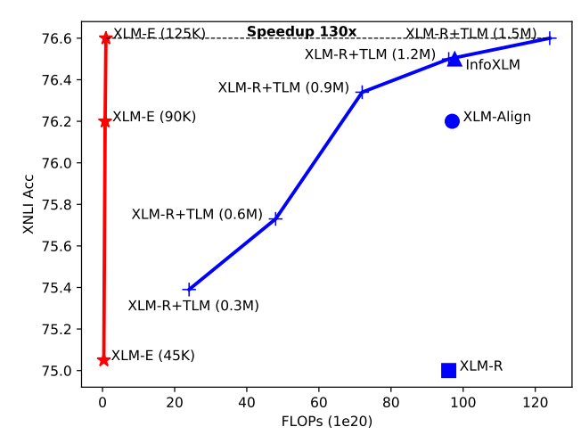
Using a pre-trained language model and then fine-tune it on downstream tasks has become a de facto trend in the field. However, these pre-training techniques such as (Masked Language Modeling (MLM), Translation Masked Modeling (TLM), ...etc.) usually requires massive computation resources. As shown in the following figure, XLM-E (red line) achieves 130x speedup compared with XLM-R augmented with TLM and around 100x speedup compared with XLM-R, XLM-Align, and InfoXLM:
Pre-training
Similar to ELECTRA, XLM-E has two Transformer components, i.e., generator and discriminator. The generator predicts the masked tokens given the masked sentence or translation pair, and the discriminator distinguishes whether the tokens are replaced by the generator. XLM-E was pre-trained on two different pre-training tasks: multilingual replaced token detection (MRTD), and translation replaced token detection (TRTD). The overall training objective is to minimize:
\[\mathcal{L} = \mathcal{L}_{\text{MLM}} + \lambda\mathcal{L}_{\text{MRTD}} + \mathcal{L}_{\text{TLM}} + \lambda\mathcal{L}_{\text{TRTD}}\]Multilingual RTD
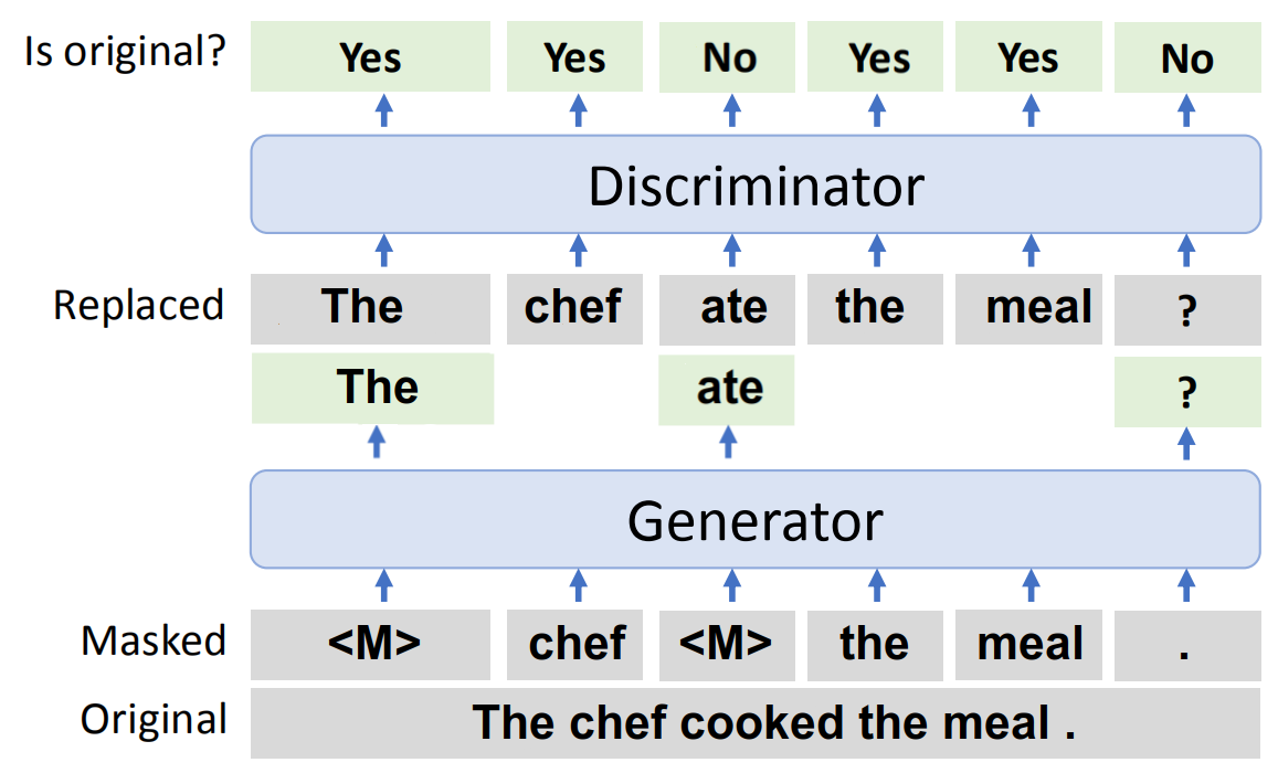
This pre-training task is a multilingual form of the Replaced Token Detection (RTD) task introduced in the ELECTRA model. Here is a small recap on RTD. The RTD task requires the model to distinguish real input tokens from corrupted multilingual sentences. The input sentences get corrupted by the generator model, and the discriminator should be able to classify the real tokens from the replaced ones as shown in the following figure:
The multilingual RTD is exactly the same with a few differences:
-
The input text can be in various languages.
-
Both the generator and the discriminator are shared across languages. The vocabulary is also shared for different languages.
-
Masking is done uniformly while it was only $15\%\ $in the ELECTRA paper.
Note:
They also tried span masking, but it significantly weakened the generator’s prediction accuracy, which in turn harmed the pre-training.
Given a input sequence $x$ that was masked using $M_{e}$ set of random positions; the loss function of the generator $G$ is:
\[\mathcal{L}_{\text{MLM}}\left( x;\ \theta_{G} \right) = - \sum_{i \in M_{e}}^{}{\text{log}\left(p_{G}\left( x_{i} \middle| x^{\text{masked}} \right) \right)}\]The loss function of the discriminator $D$ is the following; knowing that $n$ is the length of $x$ and $r_{i}$ is the label of the output (1 for “yes” and 0 for “No”):
\[\mathcal{L}_{\text{MRTD}}\left( x;\theta_{D} \right) = - \sum_{i = 1}^{n}{\log\left( p_{D}\left( r_{i} \middle| x^{\text{corrupt}} \right) \right)}\]Translation RTD
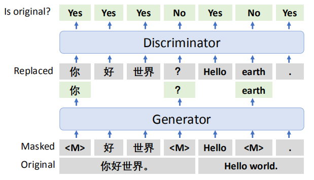
Translation RTD is a novel discriminative pre-training task which aims to distinguish real input tokens from the translation pairs concatenated together. An input translation pair $\left( e,f \right)$ gets concatenated together into a single sentence and then treated the same way as MRTD as shown in the following figure:
Given a concatenated translation pair $\left\lbrack e;f \right\rbrack$ that was masked using $M_{e}$ and $M_{f}$ sets of random positions for $e$ and $f$ respectively, the loss function of the generator $G$ is:
\[\mathcal{L}_{\text{TLM}}\left( e,f;\theta_{G} \right) = - \sum_{i \in M_{e}}^{}{\log\left( p_{G}\left( e_{i} \middle| \left\lbrack e;f \right\rbrack^{\text{masked}} \right) \right)}\] \[\ \ \ \ \ \ \ \ \ \ \ \ \ \ \ \ \ \ \ \ \ - \sum_{i \in M_{f}}^{}{\log\left( p_{G}\left( f_{i} \middle| \left\lbrack e;f \right\rbrack^{\text{masked}} \right) \right)}\]The loss function of the discriminator $D$ is the following; knowing that $n$ is the length of the concatenation and $r_{i}$ is the label of the output (1 for “yes” and 0 for “No”):
\[\mathcal{L}_{\text{TRTD}}\left( e,f;\theta_{D} \right) = - \sum_{i = 1}^{n}{\log\left( p_{D}\left( r_{i} \middle| \left\lbrack e;f \right\rbrack^{\text{corrupt}} \right) \right)}\]Note:
The generators in these pre-training tasks act like language models. That’s why their loss functions were marked as $\mathcal{L}_{\text{MLM}}$ and $\mathcal{L}_{\text{TLM}}$.
Gated Relative Position Bias
In this paper, they proposed to use gated relative position bias inspired by the GRU cells, in the self-attention mechanism. First, let’s recap how the self-attention mechanism works. Given, input tokens $\left\{ x_{1},\ …x_{n} \right\}$, the self-attention mechanism uses $q_{i}$, $k_{i}$, and $v_{i}$ for each input to compute the head output ${\widetilde{h}}_{i}$ as shown below:
\[{\widetilde{h}}_{i} = \text{softmax}\left\lbrack \frac{q_{i}W_{i}^{Q}\left( k_{i}W_{i}^{K} \right)^{T}}{\sqrt{d_{k}}} \right\rbrack v_{i}W_{i}^{V}\]Where $W_{i}^{Q},W_{i}^{K} \in \mathbb{R}^{d_{m} \times d_{k}},W_{i}^{V} \in \mathbb{R}^{d_{m} \times d_{v}}$ are learned matrices. In this paper, the self-attention output is slightly different as shown below:
\[{\widetilde{h}}_{i} = \text{softmax}\left\lbrack \frac{q_{i}W_{i}^{Q}\left( k_{i}W_{i}^{K} \right)^{T}}{\sqrt{d_{k}}} + b_{i - j} \right\rbrack v_{i}W_{i}^{V}\]Where $b_{i - j}$ denotes the gated relative position bias which is computed via:
\[g^{\left( \text{update} \right)},\ g^{\left( \text{reset} \right)} = \sigma\left( q_{i}\text{.u} \right),\ \sigma\left( q_{i}\text{.v} \right)\] \[b_{i - j} = d_{i - j} + g^{\left( \text{update} \right)}d_{i - j} + \left( 1 - g^{\left( \text{update} \right)} \right).wg^{\left( \text{reset} \right)}d_{i - j}\]Where $d_{i - j}$ is learnable relative position bias, the vectors $u,\ v \in \mathbb{R}^{d_{k}}$ are parameters, σ is the sigmoid function, and $w \in \mathbb{R}$ is a learnable value.
Results
In the following experiments, they used a 12-layer Transformer as the discriminator, with hidden size of 768, and FFN hidden size of 3,072 while they used a 4-layer Transformer as the discriminator using the same hyper-parameters. They used the same vocabulary with XLM-R that consists of 250K subwords tokenized by SentencePiece.
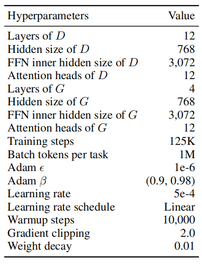
They jointly pre-trained the generator and the discriminator using Adam optimizer for 125K training steps with a dynamic batching of approximately 1M tokens. $\lambda$ was set to $50$. Check the following table for the full list of pre-training hyper-parameters.
For pre-training, they used the CC-100 dataset for the MRTD task which contains texts in 100 languages collected from CommonCrawl. They used parallel corpora in 100 languages, collected from MultiUN, IIT Bombay, OPUS, WikiMatrix, and CCAligned, for the TRTD task. For sampling, they used temperature sampling of $T = \frac{10}{7}$.
After pre-training the XLM-E model was fine-tuned on various tasks from the XTREME benchmark. The following table shows the hyper-parameters used when fine-tuning. The XTREME benchmark contains seven cross-lingual understanding tasks, namely part-of-speech tagging (POS) on the Universal Dependencies v2.5, NER named entity recognition on the Wikiann dataset, cross-lingual natural language inference on XNLI, cross-lingual paraphrase adversaries from word scrambling (PAWS-X), and cross-lingual question answering on MLQA, XQuAD, and TyDiQA-GoldP.

The following table shows the evaluation results on XTREME benchmark knowing that results of XLM-E and XLM-R~base~ are averaged over five runs.
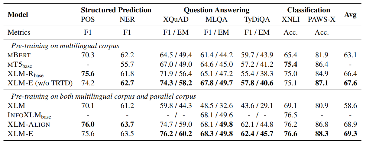
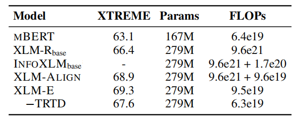
As seen from the previous table, XLM-E outperforms previous models on Question Answering and Classification problems while achieves competitive performance of Structured Predictions. All of that while uses substantially less computation:
